A team of academics entered a competition and won. Google recognized the significance of their discovery and acqui-hired them, jump-starting the commercial aspects of the field. JL
Timothy Lee reports in ars technica:
A 2013 paper described
how Google was using deep convolutional networks to read address
numbers from photos in Google Street View images. "Our system helped
us extract close to 100 million physical street numbers from Street
View imagery," the authors wrote. Researchers found that the
performance of neural networks kept improving as they got deeper. "We
find that the performance of this approach increases with the depth of
the convolutional network, with the best performance occurring in the
deepest architecture we trained."
Right now, I can open up Google Photos, type "beach," and see my photos from various beaches I've visited over the last decade. I never went through my photos and labeled them; instead, Google identifies beaches based on the contents of the photos themselves. This seemingly mundane feature is based on a technology called deep convolutional neural networks, which allows software to understand images in a sophisticated way that wasn't possible with prior techniques.
In recent years, researchers have found that the accuracy of the software gets better and better as they build deeper networks and amass larger data sets to train them. That has created an almost insatiable appetite for computing power, boosting the fortunes of GPU makers like Nvidia and AMD. Google developed its own custom neural networking chip several years ago, and other companies have scrambled to follow Google's lead.
Over at Tesla, for instance, the company has put deep learning expert Andrej Karpathy in charge of its Autopilot project. The carmaker is now developing a custom chip to accelerate neural network operations for future versions of Autopilot. Or, take Apple: the A11 and A12 chips at the heart of recent iPhones include a "neural engine" to accelerate neural network operations and allow better image- and voice-recognition applications.Experts I talked to for this article trace the current deep learning boom to one specific paper: AlexNet, nicknamed after lead author Alex Krizhevsky.
"In my mind, 2012 was the milestone year when that AlexNet paper came out," said Sean Gerrish, a machine learning expert and the author of How Smart Machines Think.
Prior to 2012, deep neural networks were something of a backwater in the machine learning world. But then Krizhevsky and his colleagues at the University of Toronto submitted an entry to a high-profile image recognition contest that was dramatically more accurate than anything that had been developed before. Almost overnight, deep neural networks became the leading technique for image recognition. Other researchers using the technique soon demonstrated further leaps in image recognition accuracy.
In this piece we'll dig deep into deep learning. I'll explain what neural networks are, how they're trained, and why they require so much computing power. And then I'll explain why a particular type of neural network—deep, convolutional networks—is so remarkably good at understanding images. And don't worry—there will be a lot of pictures.
A simple example with a single neuron
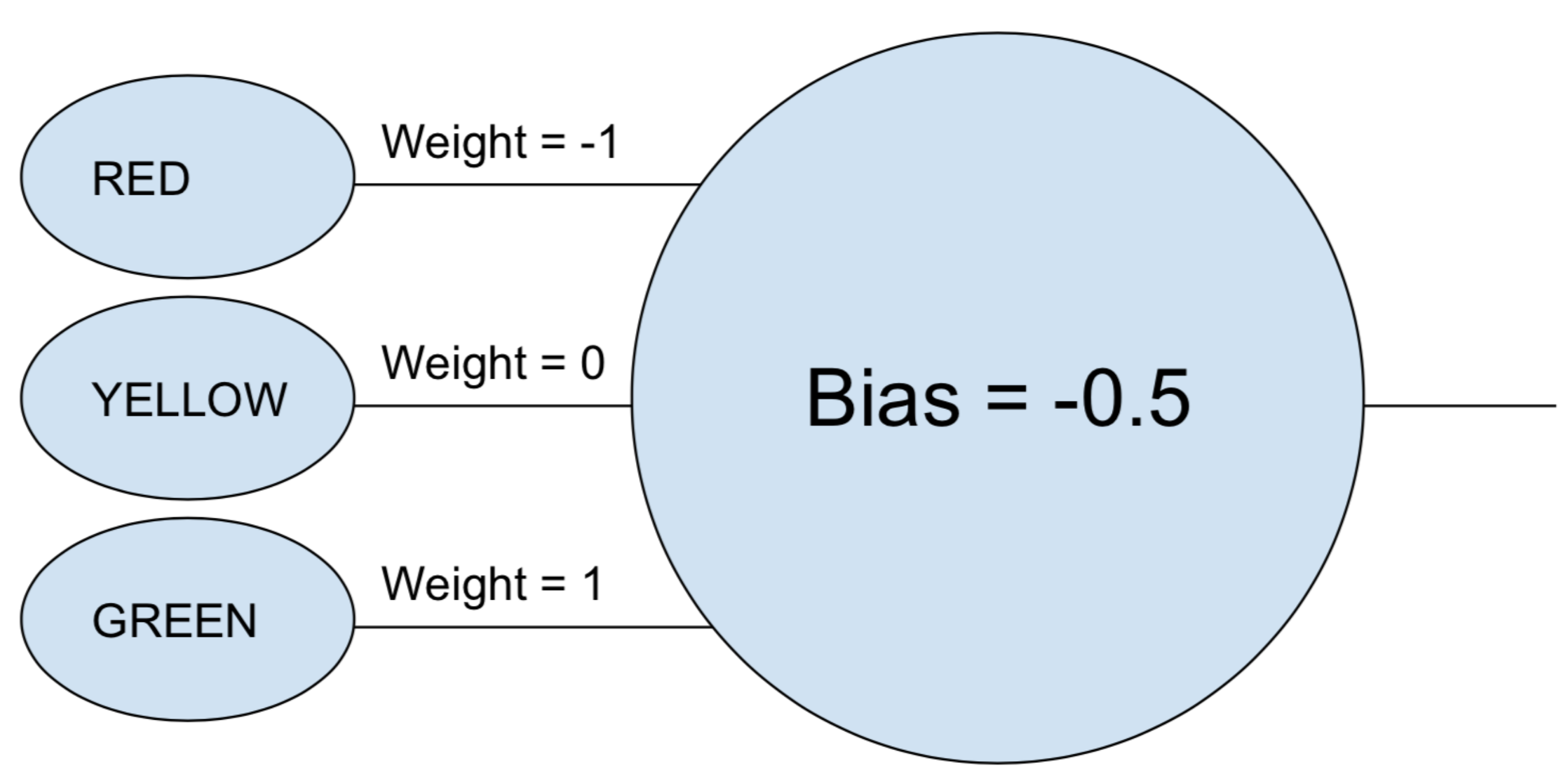
The phrase "neural network" may still feel a bit nebulous, so let's start with a simple example. Suppose you want a neural network to decide whether a car should go based on the green, yellow, and red lights of a stoplight. A neural network could accomplish this task with a single neuron.
The neuron takes each input (1 for on, 0 for off), multiplies it by its associated weight, and adds all the weighted values together. The neuron then adds the bias, which determines a threshold for the neuron to "activate." In this case, if the output is positive, we consider the neuron to have "fired"—otherwise we don't. This neuron is equivalent to the inequality "green - red - 0.5 > 0." If that evaluates to true—meaning the green light is on and the red light is off—then the car should go.
In real neural networks, artificial neurons take one additional step. After summing the weighted inputs and adding in the bias, the neuron then applies a non-linear activation function. A popular choice is the sigmoid function, an S-shaped function that always produces a value between 0 and 1.
The use of an activation function wouldn't change the result of our simple stoplight model (except we'd need to use a threshold of 0.5 instead of 0). But the nonlinearity of activation functions is essential for enabling neural networks to model more complex functions. Without an activation function, every neural network, no matter how complex, would be reducible to a linear combination of its inputs. And a linear function can't model complex real-world phenomena. Non-linear activation functions make it possible for neural networks to approximate any mathematical function.
An example network
There are lots of ways to approximate functions, of course. What makes neural networks special is that we know how to "train" them using a bit of calculus, a bunch of data, and a whole lot of computing power. Instead of having a human programmer directly design a neural network for a particular task, we can build software that starts with a fairly generic neural network, looks at a bunch of labeled examples, and then modifies the neural network so that it produces the correct label for as many of the labeled examples as possible. The hope is that the resulting network will generalize, producing the correct labels for examples previously not in its training set.
The process to get to this point started well before AlexNet. In 1986, a trio of researchers published a landmark paper about backpropagation, a technique that helped make it mathematically tractable to train complex neural networks.
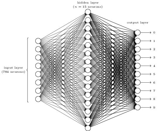
To get an intuition for how backpropagation works, let's look at a simple neural network described by Michael Nielsen in his excellent online deep learning textbook. The goal of this network is to take a 28×28 pixel image representing a handwritten digit and correctly identify whether the digit is a 0, 1, 2, etc.
Each image has 28×28=784 input values, each a real number between zero and one representing how light or dark a pixel is. Nielsen constructed a neural network that looked like this:
Micheal Nielsen
In this image, each of the circles in the middle and right columns is a neuron like the one we looked at in the previous section. Each neuron takes a weighted average of its inputs, adds a bias value, and then applies an activation function. Note that the circles on the left are not neurons—these circles represent the network's input values. While the image only shows 8 input circles, there are actually 784 inputs—one for each pixel in the input images.
Each of the 10 neurons on the right is supposed to "light up" for a different digit: the top neuron should fire when the input image is a handwritten 0 (and not otherwise), the second one should fire when the network sees a handwritten 1 (and not otherwise), and so forth.
Each neuron takes inputs from every neuron in the layer before it. So each of the 15 neurons in the middle layer has 784 input values. Each of these 15 neurons has a weight parameter for each of its 784 inputs. That means this layer alone has 15×784=11,760 weight parameters. Similarly, the output layer contains 10 neurons, each of which takes an input from each of the 15 neurons in the middle layer, adding another 15×10=150 weight parameters. On top of that, the network also has 25 bias variables—one for each of the 25 neurons.
Training the neural network
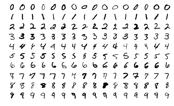
The goal of training is to tune these 11,935 parameters to maximize the chances that the correct output neuron—and only that output neuron—will light up when shown an image of a handwritten digit. We can do this using a well-known dataset called MNIST that provides 60,000 labeled 28×28 pixel images:
This image shows 160 of the 60,000 images in the MNIST dataset.
Nielsen shows how to train this network using just 74 lines of regular Python code—no special machine learning libraries needed. Training starts by choosing random values for each of those 11,935 weight and bias parameters. The software then goes through the example images, completing a two-step process for each one:
The feed-forward step computes the network's output values, given the input image and the network's current parameters.
The backpropagation step computes how much the results diverged from the correct output values, then modifies the network's parameters to slightly improve its performance on that particular input image.
Here's an example. Suppose the network is shown this image:
If the network is well-calibrated, then the network's "7" output should be close to 1, while the network's other nine outputs should all be close to 0. But suppose instead that the network's "0" output is 0.8 when shown this image. That's too high! The training algorithm will change the input weights of the "0" output neuron to get it closer to 0 next time it's shown that particular image.
To do this, the backpropagation algorithm computes an error gradient for each input weight parameter. This is a measure of how much the output error would change for a given change in the input weight. The algorithm then uses this gradient to decide how much to change each input weight—the bigger the gradient, the more that parameter is changed.
In other words, the training process "teaches" neurons in the output layer to pay less attention to inputs (which is to say neurons in the middle layer) that push them toward the wrong answer and to pay more attention to inputs that push them in the right direction.
The algorithm repeats this step for each of the other output neurons. It reduces weights of inputs for the "1," "2," "3," "4," "5," "6," "8," and "9" neurons (but not the "7" neuron) to push the value of these output neurons downward. The higher an input's value, the larger the gradient of the output error with respect to that input's weight parameter—hence the more its weight will be reduced.
Conversely, the training algorithm increases the weights of inputs to the "7" output, which will cause that neuron to produce a higher value next time it is shown this particular image. Once again, inputs with larger values will see a larger increase in their weights, causing the "7" output neuron to pay more attention to these inputs in future rounds.
The algorithm next needs to perform the same calculation for the middle layer: change each input weight in a direction that will reduce the network's errors—again, getting the "7" output closer to 1 and the others closer to 0. But each middle neuron is an input to all 10 of the neurons in the output layer, which complicates things in two ways.
First, the error gradient for any given middle-layer input depends not only on that input value, but also on error gradients in the next layer. The algorithm is called backpropagation because error gradients from later layers in a network are propagated backwards and used (along with the chain rule from calculus) to calculate gradients in earlier layers.
Also, each middle layer neuron is an input to all ten neurons in the output layer. So the training algorithm has to compute an error gradient reflecting how a change in a particular input weight will affect the average error across all outputs.
Backpropagation is a hill-climbing algorithm: each round of the algorithm causes the outputs to be closer to the correct results for that training image—but only a little bit closer. As the algorithm looks at more and more examples, it "climbs the hill" toward an optimal set of parameters, one that correctly classifies as many training examples as possible. Achieving high accuracy requires thousands of training examples, and the algorithm may need to loop through every image in this training set dozens of times before performance stops improving.
Nielsen shows how to implement all of this with just 74 lines of Python code. Remarkably, a neural network trained with this simple program is able to recognize more than 95 percent of hand-written digits in the MNIST database. With some additional refinements, a simple two-layer neural network like this is able to recognize more than 98 percent of digits.
The AlexNet breakthrough
You might have expected the development of backpropagation in the 1980s to kick off a period of rapid progress in machine learning based on neural networks, but that's not what happened. There were some people working on the technique in the 1990s and early 2000s, of course. But interest in neural networks didn't truly take off until the early 2010s.
We can see this in the results of the ImageNet competition, an annual machine learning contest organized by Stanford computer scientist Fei-Fei Li. In each year's competition, contestants were given a common set of more than a million training images—each hand-labeled with one of about 1,000 possible categories, like "fire engine," "mushroom," or "cheetah." Contestants' software was judged on its ability to classify other images that had not been included in the training set. Programs could make multiple guesses and were considered successful if one of their first five guesses for an image matched the human-chosen label.
The competition began in 2010, and deep neural networks did not play a major role the first two years. Top teams used a variety of other machine learning techniques with fairly mediocre results. The winning team in 2010 had a top-5 error rate of 28 percent. In 2011, it was 25 percent.
Then came 2012. That team from the University of Toronto submitted an entry—the one later dubbed AlexNet after lead author Alex Krizhevsky—and blew competitors out of the water. Using a deep neural network, the team achieved a 16-percent top-five error rate. The closest rival that year had a 26-percent error rate.
The handwriting recognition network discussed above had two layers, 25 neurons, and almost 12,000 parameters. AlexNet was vastly larger and more complex: eight trainable layers, 650,000 neurons, and 60 million parameters.
Training a network of that size required massive computing power, and AlexNet was designed to take advantage of the massive parallel computing power provided by modern GPUs. The researchers figured out how to divide the work of training their network across two GPUs, giving them twice the computing power to work with. Still, despite aggressive optimization, training the network took five to six days with the hardware available in 2012 (a pair of Nvidia GTX 580 GPUs, each with 3GB of memory).
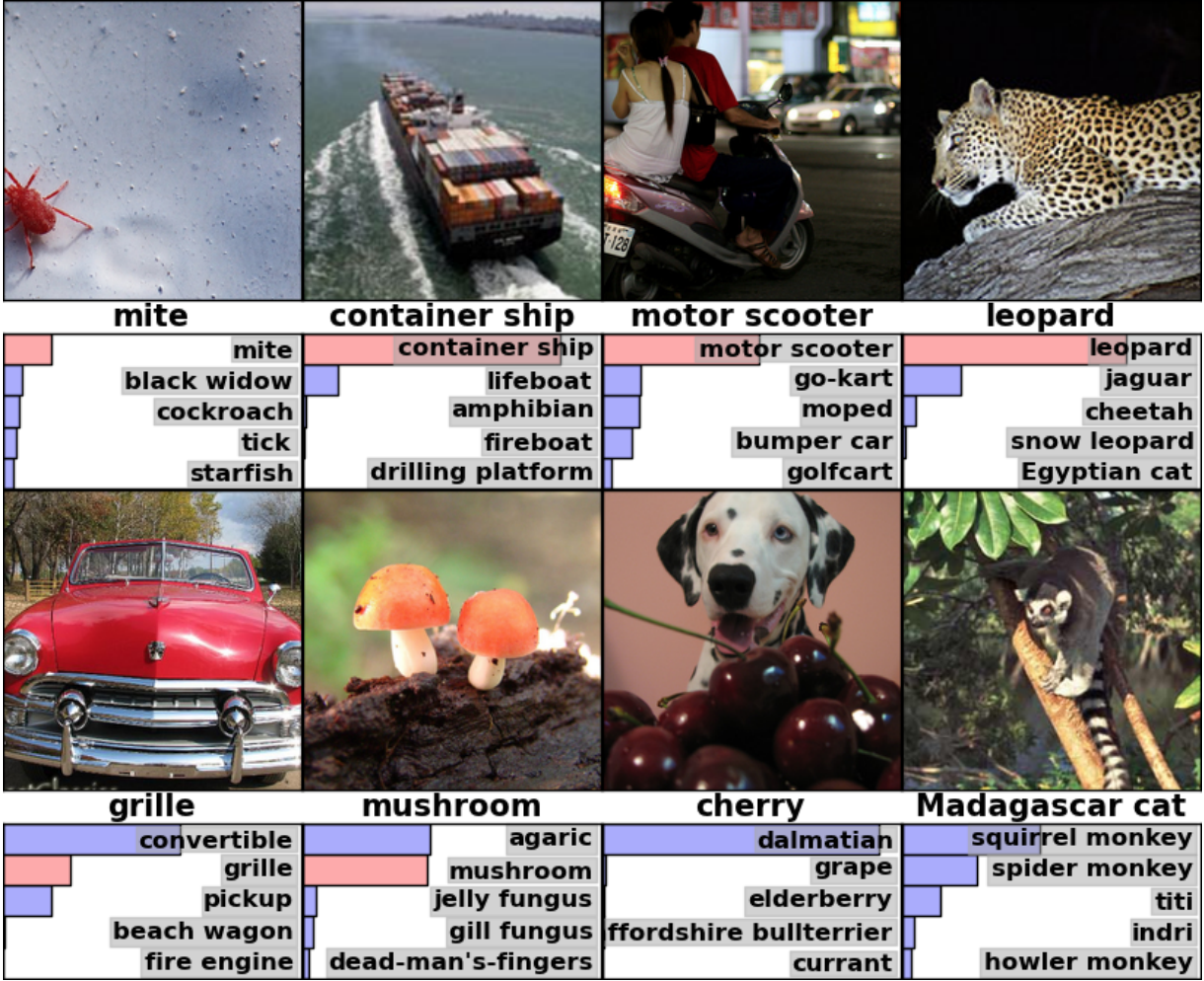
It's helpful to look at some examples of AlexNet's results to appreciate what an impressive breakthrough it was. Here's a snapshot from the paper showing a handful of images and AlexNet's top-five classifications:
AlexNet was able to recognize that the first image contained a mite even though the mite was a small shape at the very edge of the image. The software not only correctly identified the leopard, its other top guesses—jaguar, cheetah, snow leopard, and Egyptian cat—were all similar-looking cats. AlexNet labeled an image of a mushroom with "agaric"—a type of mushroom. "Mushroom," the officially correct label, was AlexNet's second choice.
AlexNet's "mistakes" were almost as impressive. It labeled a picture of a dalmatian behind some cherries with "dalmatian," whereas the official label was "cherry." AlexNet recognized that the picture contained some kind of fruit—"grape" and "elderberry" were among its top-five choices—but it didn't quite recognize that they were cherries. Shown a picture of a Madagascar cat in a tree, AlexNet listed a bunch of small tree-climbing mammals. Plenty of humans (including me) would have gotten this one wrong.
It was a truly impressive performance, demonstrating that software could recognize common objects in a wide variety of orientations and settings. Deep neural networks quickly became the most popular technique for image recognition tasks, and the machine learning world hasn't looked back since.
"Following the success of the deep learning-based method in 2012, the vast majority of entries in 2013 used deep convolutional neural networks," the ImageNet sponsors wrote. That pattern continued in subsequent years, and later winners built on the basic techniques pioneered by the AlexNet team. By 2017, contestants using much deeper neural networks had pushed the top-five error rate down below three percent. Given the complexity of the task, this arguably makes computers better at this task than many human beings.
Enlarge/ This slide from the ImageNet team shows the winning team's error rate each year in the top-5 classification task. The error rate fell steadily from 2010 to 2017.
Technically, AlexNet was a convolutional neural network. In this section I'll explain what a convolutional network does and why the technique has become crucial to modern image recognition algorithms.
The simple handwriting recognition network we explored earlier was fully connected: every neuron in the first layer is an input to every neuron in the second layer. This structure works well enough for the relatively simple task of recognizing digits on small 28×28 pixel images. But it doesn't scale well.
In the MNIST dataset of handwritten digits, characters are always centered. This greatly simplifies training because it means that (for example) a seven will always have some dark pixels at the top and at the right of the image, while the lower-left is always white. A zero will almost always have a white spot near the middle and darker pixels near the edges. A simple, fully connected network can detect these kinds of patterns fairly easily.
But suppose you wanted to build a neural network that could recognize numbers that might be located anywhere in a larger image. A fully connected network won't work as well, because it doesn't have an efficient way to recognize similarities between shapes located in different parts of the image. If your training set happened to have most of the sevens in the upper-left corner, then you'd end up with a network that is better at recognizing sevens in the upper left than elsewhere in the image.
Theoretically you could solve this problem by making sure your training set had many examples of every digit in every possible pixel position. But in practice that would be hugely wasteful. As the size of images and the depth of networks increased, the number of connections—and hence the number of input weight parameters—would explode. You'd need vastly more training images (not to mention a lot more computing power) to achieve adequate accuracy.
When a neural network learns to recognize a shape in one position within the image, it should be able to apply that learning to recognize similar shapes in other parts of the image. Convolutional neural networks provide an elegant solution to this problem.
"It's like taking a stencil or pattern and matching it against every single spot on the image," said AI researcher Jie Tang. "You have a stencil outline of a dog, and you basically match the upper-right corner of it against your stencil—is there a dog there? If not, you move the stencil a little bit. You do this over the whole image. It doesn't matter where in the image the dog appears. The stencil will match it. You don't want to have each subsection of the network learn its own separate dog classifier."
So, imagine if we took a large image and broke it into 28×28 pixel squares. Then we could feed each square into the fully connected handwriting recognition network we explored earlier. If the "7" output lit up for at least one of those squares, that's a sign that the image as a whole probably has a seven in it. This is essentially what convolutional networks do.
In convolutional networks, these "stencils" are known as feature detectors, and the area they look at is called the receptive field. Real feature detectors tend to have receptive fields much smaller than 28 pixels on a side. In AlexNet, the first convolutional layer had feature detectors whose receptive field was 11 pixels by 11 pixels. Subsequent convolutional layers in AlexNet had receptive fields three or five units wide.
As a feature detector sweeps across an input image, it produces a feature map: a two-dimensional grid that indicates how strongly the detector was activated by different parts of the image. Convolutional layers will usually have more than one feature detector, each scanning the input image for a different pattern. In AlexNet, the first layer had 96 feature detectors and produced 96 feature maps.
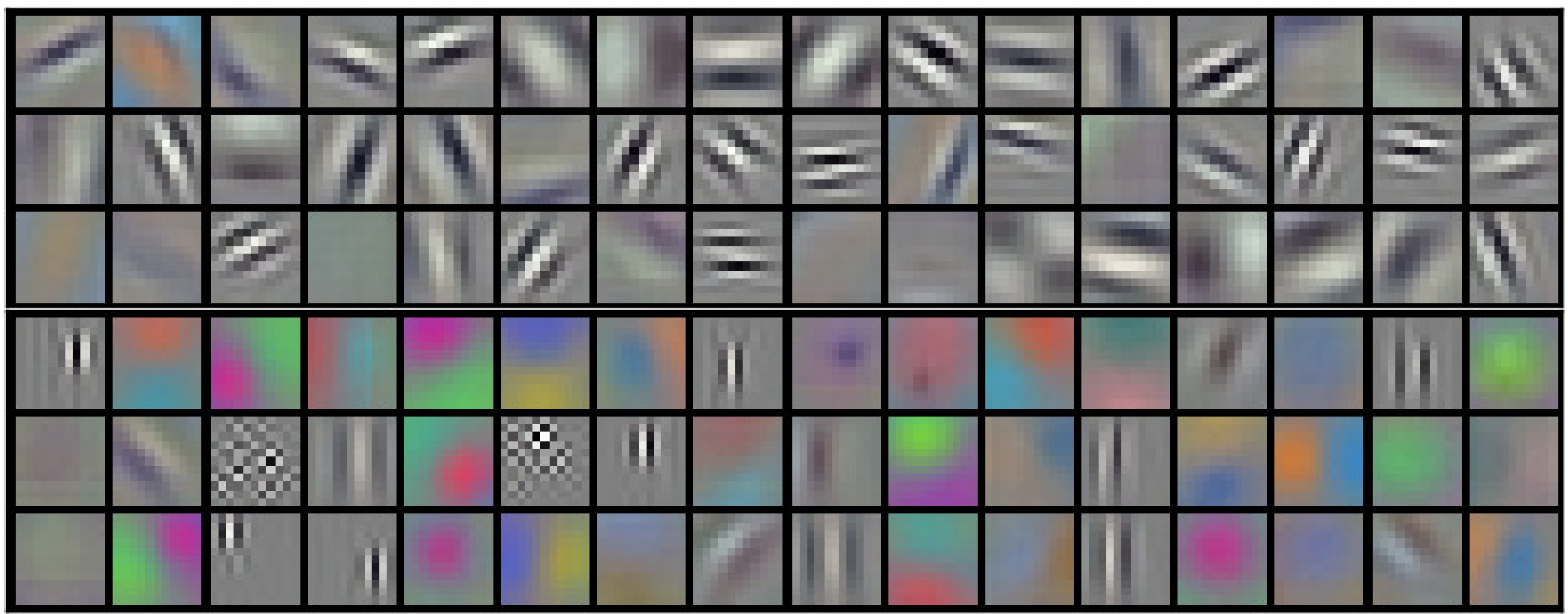
To make this more concrete, here's a visual representation of visual patterns learned by each of the 96 feature detectors in AlexNet's first layer after network training. There are detectors that look for horizontal or vertical lines, gradients from light to dark, checkerboard patterns, and many other shapes.
A color image is commonly represented as a pixel map with three numbers for each pixel: a red value, a green value, and a blue value. AlexNet's first layer takes this three-number representation of the image and transforms it into a 96-number representation. Each "pixel" in this image has 96 values, one for each of the 96 feature detectors.
In this example, the first of these 96 values indicates whether a particular point in the image matches this pattern:
The second value indicates whether a particular point matches this pattern:
The third value indicates whether a particular point matches this pattern:
... and so on for the other 93 feature detectors in AlexNet's first layer. The first layer outputs a new representation of the image where each "pixel" is a 96-number vector (as I'll explain later, this new representation is also scaled down by a factor of four).
So that's AlexNet's first layer. Next there are four more convolutional layers, each of which takes the previous layer's output for its input.
As we've seen, the first layer detects basic patterns like horizontal and vertical lines, light-to-dark gradients, and curves. The second layer then uses these as building blocks to detect slightly more complex shapes. For example, the second layer might have a feature detector that finds circles by combining the output of first-layer feature detectors that find curves. The third layer finds still more complex shapes by combining features from the second layer. The fourth and fifth layers find even more complex patterns.
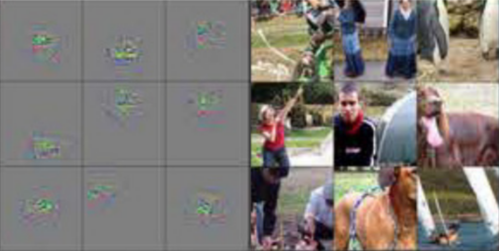
Researchers Matthew Zeiler and Rob Fergus published an excellent 2014 paper that offers some helpful ways to visualize the kinds of patterns recognized by a five-layer neural network similar to ImageNet.
In this slideshow from their paper, each image (other than the first first one) has two halves. On the right you'll see examples of thumbnail images that strongly activated a particular feature detector. These are organized into groups of nine—each group corresponds to a different feature detector. On the left is a map that shows which specific pixels within that thumbnail image were most responsible for the strong match. You can see this most dramatically in the fifth layer, as there are feature detectors that strongly light up for dogs, corporate logos, unicycle wheels, and so forth. Flipping through the images, you can see that each layer is capable of recognizing more complex patterns than the ones before it. The first layer recognizes simple pixel patterns that don't look like much at all. The second layer recognizes textures and simple shapes. By the third layer, we see recognizable shapes like car wheels and reddish-orange spheres (which might be tomatoes, ladybugs, or something else).
The first layer has a receptive field 11 units on a side, while later layers have receptive fields that are three to five units on a side. But remember, these later layers are looking at feature maps generated by the earlier layers, and each "pixel" in these feature maps represents several pixels in the original image. So each layer's receptive field encompasses a larger portion of the original image than the layers that preceded it. That's part of the reason that the thumbnail images in later layers seem more complex than those of earlier layers.
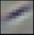
The network's fifth and final layer is able to recognize an impressively wide range of elements within these images. For example, take a look at this image, which I've plucked from the upper-right-hand corner of the layer-five image above:
The nine images on the right might not look very similar. But if you look at the nine heat maps on the left, you'll see that this particular feature detector isn't focusing on the objects in the foreground of each image. Instead, it's focusing on the grassy parts in the background of each image!
Obviously, a grass-detector is useful if one of the categories you're trying to identify is "grass," but this is likely to be useful for a lot of other categories, too. Following the five convolutional layers, AlexNet has three layers that are fully connected like the layers in our handwriting recognition network. These layers consider every one of the feature maps produced by the fifth convolutional layer as they try to classify the image into one of the 1,000 possible categories.
So if a picture has grass in the background, it's more likely to show a wild animal. On the other hand, if the picture has grass in the background, it's less likely to be a picture of indoor furniture. These and other layer-five feature detectors provide a wealth of information about what's probably in the photo. The last few layers of the network synthesize this information to produce an educated guess about what the picture as a whole depicts.
What makes convolutional layers different: Shared input weights
We've seen that the feature detectors in convolutional layers perform impressive pattern recognition, but so far I haven't explained how convolutional networks actually work.
A convolutional layer is a layer of neurons. Like any neurons, these take a weighted average of their inputs and then apply an activation function. Parameters are trained using the backpropagation techniques we've discussed.
But unlike the neural networks above, a convolutional layer isn't fully connected. Each neuron only takes input from a small fraction of the neurons in the previous layer. And, crucially, the neurons in convolutional networks have shared input weights.
Let's zoom in on the first neuron in the first convolutional layer of AlexNet. This layer has a receptive field of 11×11 pixels, so the first neuron looks at an 11×11 square of pixels in one corner of the image. This neuron takes input from these 121 pixels, and each pixel has three values—red, green, and blue. So the neuron has a total of 363 inputs. Like any neuron, this one takes a weighted average of these 363 input values and then applies an activation function. And because it has 363 input values, it also needs 363 input weight parameters.
The second neuron in AlexNet's first layer looks a lot like the first one. It also looks at an 11×11 pixel square, but its receptive field is shifted by four pixels from the first neuron's receptive field. This creates a seven-pixel overlap between the two receptive fields, which avoids having interesting patterns getting missed if they straddle the line between two neurons. This second neuron also takes the 363 values that describe its 11×11 pixel square, multiplies each value by a weight parameter, adds these values up, and applies an activation function.
Rather than having its own set of 363 input weights, the second neuron uses the same input weights as the first neuron. The upper-left pixel of the first neuron uses the same input weights as the upper-left pixel of the second neuron. So the two neurons are looking for exactly the same pattern; they just have receptive fields that are offset from each other by four pixels.
There are a lot more than two neurons of course: there are actually 3,025 neurons laid out in a 55×55 grid. Each of these 3,025 neurons uses the same set of 363 input weights as those first two neurons. Together, all of those neurons form a feature detector that "scans" for a specific pattern wherever it might be located in an image.
Remember that the first layer of AlexNet had 96 feature detectors. The 3,025 neurons I just mentioned constitute one of those 96 feature detectors. Each of the other 95 feature detectors is a different group of 3,025 neurons. Each group of 3,025 neurons shares its 363 input weights with others in its group—but not with neurons in the other 95 feature detectors.
Convolutional networks are trained using the same basic backpropagation algorithm used to train fully connected networks, but the convolutional structure makes the training process more efficient and effective.
"Using convolutions is really helpful because you can re-use parameters," machine learning expert and author Sean Gerrish told Ars. That drastically cuts down on the number of input weights the network needs to learn, which allows the network to produce better results with fewer training examples.
Learning from one part of an image can translate into better recognition of the same pattern in other locations in other images. This allows the network to achieve high performance with far fewer training examples.
People quickly realized the power of deep convolutional networks
The AlexNet paper was a sensation in the academic machine learning community, but its significance was also quickly recognized in industry. Google became particularly interested in the technique.
In 2013, Google acquired a startup formed by the authors of the AlexNet paper. They used the technology to add a new image search feature to Google Photos. "We took cutting edge research straight out of an academic research lab and launched it, in just a little over six months," wrote Google's Chuck Rosenberg.
Meanwhile, a 2013 paper described how Google was using deep convolutional networks to read address numbers from photos in Google Street View images. "Our system has helped us extract close to 100 million physical street numbers from Street View imagery," the authors wrote.
Researchers found that the performance of neural networks kept improving as they got deeper. "We find that the performance of this approach increases with the depth of the convolutional network, with the best performance occurring in the deepest architecture we trained," the Google Street View team wrote. "Our experiments suggest deeper architectures may obtain better accuracy, with diminishing returns."
So after AlexNet, neural networks kept getting deeper. A Google team submitted the winning entry to the 2014 ImageNet competition—just two years after AlexNet's win in 2012. Like AlexNet, it was based on a deep convolutional neural network, but Google used a much deeper 22-layer network to achieve a 6.7-percent top-five error rate—a big improvement over AlexNet's 16-percent error rate.
Still, deeper networks were only useful with large training sets. For this reason, Gerrish argues that the ImageNet dataset and competition played a key role in enabling the success of deep convolutional networks. Remember, the ImageNet competition gave contestants a million images and asked them to assign them to one of 1,000 different categories.
"Having a million images to train your network means that there are 1,000 images per class," Gerrish said. Without such a large dataset, he said, "you would have had too many parameters to train a network."
Recent years have brought a continued focus on amassing larger data in order to train deeper, more accurate networks. It's a big reason why self-driving car companies have focused so much on racking up miles on public roads—images and video from testing are sent back to headquarters and used to train the companies' image recognition networks.
The discovery that deeper networks and larger training sets could deliver better and better performance has created an insatiable demand for more computing power. A big part of AlexNet's success was the realization that neural network training involved matrix operations that could be performed efficiently using the highly parallel computational power of a graphics card.
"Neural networks are parallelizable," said machine learning researcher Jie Tang. Graphics cards—which provide massively parallel computing power for video games—turned out to be useful for neural networks.
"The core operation of GPUs, really fast matrix multiplication, ended up being the core operation of neural nets," Tang said.
That has turned into a bonanza for Nvidia and AMD, the leading GPU makers. Both companies have worked to develop new chips that are tuned for the unique needs of machine learning applications, and AI applications now account for a significant fraction of these companies' GPU sales.
In 2016, Google announced that it had created a custom chip called a Tensor Processing Unit (TPU) specifically for neural network operations. "Although Google considered building an Application-Specific Integrated Circuit (ASIC) for neural networks as early as 2006, the situation became urgent in 2013, Google wrote last year. "That’s when we realized that the fast-growing computational demands of neural networks could require us to double the number of data centers we operate."
Initially, access to TPUs was limited to Google's own proprietary services, but Google later began to allow anyone to use the technology via Google's cloud computing platform.
Of course, Google isn't the only company working on AI chips. For just a small sampling: recent versions of the iPhone's chips include a "neural engine" optimized for neural network operations. Intel is developing its own line of chips optimized for deep learning. Tesla announced recently that it was dumping Nvidia's chips in favor of a homebrew neural network chip. Amazon is reportedly working on an AI chip of its own, too.
Why deep neural networks are hard to understand
I've explained how deep neural networks work, but I haven't really explained why they work as well as they do. It's more than a little mysterious how a mind-bogglingly large number of matrix calculations could enable a computer system to distinguish a jaguar from a cheetah and an elderberry from a currant.
Perhaps the most remarkable thing about neural networks is what they don't do. Convolutions allow neural networks to understand translations—they can tell if a pattern in the upper-right corner of one image is similar to a pattern in the upper-left corner of another.
But beyond that, convolutional networks have no real understanding of geometry. They can't recognize that one image is similar to another if it's rotated by 45 degrees or scaled up by a factor of two. Convolutional networks make no attempt to understand three-dimensional object structures, and they can't correct for varying lighting conditions.
Yet deep neural networks can recognize pictures of dogs whether they're taken from the front or the side, and whether they take up a small part of the image or a large one. How do they do that? It turns out that with enough data, a brute-force statistical approach is good enough to get the job done. A convolutional network isn't designed to "imagine" how a particular image would look if viewed from a different angle or in different circumstances, but with enough labeled examples, it can learn all possible permutations by sheer repetition.
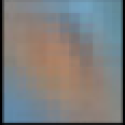
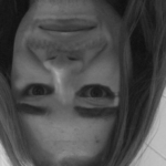
There's evidence that the human visual system actually works in a similar way. Consider this pair of pictures (make sure you look carefully at the first image before flipping to the second on it.
Obviously, the creator of this image took someone's image and flipped the eyes and mouth upside down. The image looks relatively normal when you look at it upside down because the human visual system is used to seeing eyes and mouths in this orientation. But when you look at the face right-side up, the face immediately looks freakishly misshapen.
This suggests that the human visual system relies on some of the same crude pattern-matching techniques that neural networks do. If we're looking at something that's almost always viewed in one orientation—like human eyes—we're much better at recognizing them in their usual orientation.
Neural networks are good at using all of the context in a picture to figure out what it shows. For example, cars usually appear on roads. Dresses usually appear either on women's bodies or hanging in closets. Airplanes either appear framed against a blue sky or taxiing on a runway. Nobody explicitly teaches neural networks these correlations, but with enough labeled examples the network can learn them automatically.
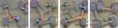
In 2015, some Google researchers tried to understand neural networks better by "running them backwards." Instead of using pictures to train neural networks, they used a trained neural network to modify images. For example, they started with an image that contained random noise and then gradually modified it to strongly "light up" one of the outputs of a neural network—effectively asking the neural network to "draw" one of the categories it had been trained to recognize. In one fascinating case, they had a neural network generate pictures that would strongly activate a neural network that had been trained to recognize dumbbells.
"There are dumbbells in there alright, but it seems no picture of a dumbbell is complete without a muscular weightlifter there to lift them," the Google researchers wrote.
Again, this might seem weird at first glance, but it's not actually that different from what humans do. If we see a small or blurry object in an image, we look at the surrounding environment for clues about what might be going on in the picture. Humans obviously reason about images in different ways, drawing on our sophisticated conceptual understanding of the world around us. But ultimately, deep neural networks are good at image recognition because they take full advantage of all the context shown in a picture, which isn't that different from how human beings do it.
As a Partner and Co-Founder of Predictiv and PredictivAsia, Jon specializes in management performance and organizational effectiveness for both domestic and international clients. He is an editor and author whose works include Invisible Advantage: How Intangilbles are Driving Business Performance. Learn more...


0 comments:
Post a Comment